Mouse CNS Sample Integration Tutorial
Creator: Sebastian Birk (sebastian.birk@helmholtz-munich.de).
Affiliation: Helmholtz Munich, Institute of AI for Health (AIH), Talavera-López Lab
Date of Creation: 18.05.2023
Date of Last Modification: 21.08.2024
In this tutorial we apply NicheCompass to integrate three samples (sagittal brain sections) of the STARmap PLUS mouse central nervous system dataset / atlas from Shi, H. et al. Spatial atlas of the mouse central nervous system at molecular resolution. Nature 622, 552–561 (2023).
Sample 1 has:
91,246 observations at cellular resolution with cell type annotations
1022 probed genes
Sample 2 has:
123,836 observations at cellular resolution with cell type annotations
1022 probed genes
Sample 3 has:
207,591 observations at cellular resolution with cell type annotations
1022 probed genes
Check the documentation for NicheCompass installation instructions.
The data for this tutorial can be downloaded from Google Drive. It has to be stored under
<repository_root>/data/spatial_omics/.starmap_plus_mouse_cns_batch1.h5ad
starmap_plus_mouse_cns_batch2.h5ad
starmap_plus_mouse_cns_batch3.h5ad
A pretrained model to run only the analysis can be downloaded from Google Drive. It has to be stored under
<repository_root>/artifacts/single_sample/<timestamp>/model/.<timestamp>: 22082024_000607
1. Setup
1.1 Import Libraries
%load_ext autoreload
%autoreload 2
import os
import random
import warnings
from datetime import datetime

import anndata as ad
import gdown
import matplotlib.pyplot as plt
import numpy as np
import pandas as pd
import scanpy as sc
import scipy.sparse as sp
import seaborn as sns
import squidpy as sq
from matplotlib import gridspec
from sklearn.preprocessing import MinMaxScaler

from nichecompass.models import NicheCompass
from nichecompass.utils import (add_gps_from_gp_dict_to_adata,
                                create_new_color_dict,
                                compute_communication_gp_network,
                                visualize_communication_gp_network,
                                extract_gp_dict_from_mebocost_ms_interactions,
                                extract_gp_dict_from_nichenet_lrt_interactions,
                                extract_gp_dict_from_omnipath_lr_interactions,
                                filter_and_combine_gp_dict_gps_v2,
                                generate_enriched_gp_info_plots)
1.2 Define Parameters
### Dataset ###
dataset = "starmap_plus_mouse_cns"
species = "mouse"
batches = ["batch1", "batch2", "batch3"]
spatial_key = "spatial"
n_neighbors = 4

### Model ###
# AnnData keys
counts_key = "counts"
adj_key = "spatial_connectivities"
cat_covariates_keys = ["batch"]
gp_names_key = "nichecompass_gp_names"
active_gp_names_key = "nichecompass_active_gp_names"
gp_targets_mask_key = "nichecompass_gp_targets"
gp_targets_categories_mask_key = "nichecompass_gp_targets_categories"
gp_sources_mask_key = "nichecompass_gp_sources"
gp_sources_categories_mask_key = "nichecompass_gp_sources_categories"
latent_key = "nichecompass_latent"

# Architecture
cat_covariates_embeds_injection = ["gene_expr_decoder"]
cat_covariates_embeds_nums = [3]
cat_covariates_no_edges = [True]
conv_layer_encoder = "gcnconv" # change to "gatv2conv" if enough compute and memory
active_gp_thresh_ratio = 0.01

# Trainer
n_epochs = 400
n_epochs_all_gps = 25
lr = 0.001
lambda_edge_recon = 500000.
lambda_gene_expr_recon = 300.
lambda_l1_masked = 0. # prior GP  regularization
lambda_l1_addon = 30. # de novo GP regularization
edge_batch_size = 4096 # increase if more memory available or decrease to save memory
n_sampled_neighbors = 4
use_cuda_if_available = True

### Analysis ###
cell_type_key = "Main_molecular_cell_type"
latent_leiden_resolution = 0.2
latent_cluster_key = f"latent_leiden_{str(latent_leiden_resolution)}"
sample_key = "batch"
spot_size = 0.2
differential_gp_test_results_key = "nichecompass_differential_gp_test_results"
1.3 Run Notebook Setup
warnings.filterwarnings("ignore")
# Get time of notebook execution for timestamping saved artifacts
now = datetime.now()
current_timestamp = now.strftime("%d%m%Y_%H%M%S")
1.4 Configure Paths
# Define paths
ga_data_folder_path = "../../../data/gene_annotations"
gp_data_folder_path = "../../../data/gene_programs"
so_data_folder_path = "../../../data/spatial_omics"
omnipath_lr_network_file_path = f"{gp_data_folder_path}/omnipath_lr_network.csv"
collectri_tf_network_file_path = f"{gp_data_folder_path}/collectri_tf_network_{species}.csv"
nichenet_lr_network_file_path = f"{gp_data_folder_path}/nichenet_lr_network_v2_{species}.csv"
nichenet_ligand_target_matrix_file_path = f"{gp_data_folder_path}/nichenet_ligand_target_matrix_v2_{species}.csv"
mebocost_enzyme_sensor_interactions_folder_path = f"{gp_data_folder_path}/metabolite_enzyme_sensor_gps"
gene_orthologs_mapping_file_path = f"{ga_data_folder_path}/human_mouse_gene_orthologs.csv"
artifacts_folder_path = f"../../../artifacts"
model_folder_path = f"{artifacts_folder_path}/sample_integration/{current_timestamp}/model"
figure_folder_path = f"{artifacts_folder_path}/sample_integration/{current_timestamp}/figures"
1.5 Create Directories
os.makedirs(model_folder_path, exist_ok=True)
os.makedirs(figure_folder_path, exist_ok=True)
os.makedirs(so_data_folder_path, exist_ok=True)
1.6 Download Files (Optional)
You can skip this part if you have downloaded the files mentioned above manually, or you are using your own data.
gdown.download("https://drive.google.com/uc?id=1MOjIyue7a-JDAcnAseqIljDyoO7KtH99", so_data_folder_path+'/starmap_plus_mouse_cns_batch1.h5ad')
gdown.download("https://drive.google.com/uc?id=1_RcLVuZcJiFw-iaB7saPX4ydR1X2CvaS", so_data_folder_path+'/starmap_plus_mouse_cns_batch2.h5ad')
gdown.download("https://drive.google.com/uc?id=1sIIHGZ55aYBbgCXCBvIrGxB7i7OgUuJ9", so_data_folder_path+'/starmap_plus_mouse_cns_batch3.h5ad')
2. Prepare Model Training
2.1 Create Prior Knowledge Gene Program (GP) Mask
NicheCompass expects a prior GP mask as input, which it will use to make its latent feature space interpretable (through linear masked decoders).
The user can provide a custom GP mask to NicheCompass based on the biological question of interest.
As a default, here we create a GP mask based on three databases of prior knowledge of inter- and intracellular interaction pathways:
OmniPath (Ligand-Receptor GPs)
MEBOCOST (Enzyme-Sensor GPs)
NicheNet (Combined Interaction GPs)
# Retrieve OmniPath GPs (source: ligand genes; target: receptor genes)
omnipath_gp_dict = extract_gp_dict_from_omnipath_lr_interactions(
    species=species,
    load_from_disk=False,
    save_to_disk=True,
    lr_network_file_path=omnipath_lr_network_file_path,
    gene_orthologs_mapping_file_path=gene_orthologs_mapping_file_path,
    plot_gp_gene_count_distributions=True,
    gp_gene_count_distributions_save_path=f"{figure_folder_path}" \
                                           "/omnipath_gp_gene_count_distributions.svg")
# Display example OmniPath GP
omnipath_gp_names = list(omnipath_gp_dict.keys())
random.shuffle(omnipath_gp_names)
omnipath_gp_name = omnipath_gp_names[0]
print(f"{omnipath_gp_name}: {omnipath_gp_dict[omnipath_gp_name]}")
# Retrieve NicheNet GPs (source: ligand genes; target: receptor genes, target genes)
nichenet_gp_dict = extract_gp_dict_from_nichenet_lrt_interactions(
    species=species,
    version="v2",
    keep_target_genes_ratio=1.,
    max_n_target_genes_per_gp=250,
    load_from_disk=False,
    save_to_disk=True,
    lr_network_file_path=nichenet_lr_network_file_path,
    ligand_target_matrix_file_path=nichenet_ligand_target_matrix_file_path,
    gene_orthologs_mapping_file_path=gene_orthologs_mapping_file_path,
    plot_gp_gene_count_distributions=True)
# Display example NicheNet GP
nichenet_gp_names = list(nichenet_gp_dict.keys())
random.shuffle(nichenet_gp_names)
nichenet_gp_name = nichenet_gp_names[0]
print(f"{nichenet_gp_name}: {nichenet_gp_dict[nichenet_gp_name]}")
# Retrieve MEBOCOST GPs (source: enzyme genes; target: sensor genes)
mebocost_gp_dict = extract_gp_dict_from_mebocost_ms_interactions(
    dir_path=mebocost_enzyme_sensor_interactions_folder_path,
    species=species,
    plot_gp_gene_count_distributions=True)
# Display example MEBOCOST GP
mebocost_gp_names = list(mebocost_gp_dict.keys())
random.shuffle(mebocost_gp_names)
mebocost_gp_name = mebocost_gp_names[0]
print(f"{mebocost_gp_name}: {mebocost_gp_dict[mebocost_gp_name]}")
# Filter and combine GPs
gp_dicts = [omnipath_gp_dict, nichenet_gp_dict, mebocost_gp_dict]
combined_gp_dict = filter_and_combine_gp_dict_gps_v2(
    gp_dicts,
    verbose=True)

print(f"Number of gene programs after filtering and combining: "
      f"{len(combined_gp_dict)}.")
2.2 Load Data & Compute Spatial Neighbor Graph
NicheCompass expects a precomputed spatial adjacency matrix stored in ‘adata.obsp[adj_key]’.
The user can customize the spatial neighbor graph construction based on the biological question of interest.
In the sample integration setting, we will compute a separate spatial adjacency matrix for each sample and combine them as disconnected components.
adata_batch_list = []

for batch in batches:
    print(f"Processing batch {batch}...")
    print("Loading data...")
    adata_batch = sc.read_h5ad(
        f"{so_data_folder_path}/{dataset}_{batch}.h5ad")

    print("Computing spatial neighborhood graph...\n")
    # Compute (separate) spatial neighborhood graphs
    sq.gr.spatial_neighbors(adata_batch,
                            coord_type="generic",
                            spatial_key=spatial_key,
                            n_neighs=n_neighbors)

    # Make adjacency matrix symmetric
    adata_batch.obsp[adj_key] = (
        adata_batch.obsp[adj_key].maximum(
            adata_batch.obsp[adj_key].T))
    adata_batch_list.append(adata_batch)
adata = ad.concat(adata_batch_list, join="inner")

# Combine spatial neighborhood graphs as disconnected components
batch_connectivities = []
len_before_batch = 0
for i in range(len(adata_batch_list)):
    if i == 0: # first batch
        after_batch_connectivities_extension = sp.csr_matrix(
            (adata_batch_list[0].shape[0],
            (adata.shape[0] -
            adata_batch_list[0].shape[0])))
        batch_connectivities.append(sp.hstack(
            (adata_batch_list[0].obsp[adj_key],
            after_batch_connectivities_extension)))
    elif i == (len(adata_batch_list) - 1): # last batch
        before_batch_connectivities_extension = sp.csr_matrix(
            (adata_batch_list[i].shape[0],
            (adata.shape[0] -
            adata_batch_list[i].shape[0])))
        batch_connectivities.append(sp.hstack(
            (before_batch_connectivities_extension,
            adata_batch_list[i].obsp[adj_key])))
    else: # middle batches
        before_batch_connectivities_extension = sp.csr_matrix(
            (adata_batch_list[i].shape[0], len_before_batch))
        after_batch_connectivities_extension = sp.csr_matrix(
            (adata_batch_list[i].shape[0],
            (adata.shape[0] -
            adata_batch_list[i].shape[0] -
            len_before_batch)))
        batch_connectivities.append(sp.hstack(
            (before_batch_connectivities_extension,
            adata_batch_list[i].obsp[adj_key],
            after_batch_connectivities_extension)))
    len_before_batch += adata_batch_list[i].shape[0]
adata.obsp[adj_key] = sp.vstack(batch_connectivities)
2.3 Add GP Mask to Data
# Add the GP dictionary as binary masks to the adata
add_gps_from_gp_dict_to_adata(
    gp_dict=combined_gp_dict,
    adata=adata,
    gp_targets_mask_key=gp_targets_mask_key,
    gp_targets_categories_mask_key=gp_targets_categories_mask_key,
    gp_sources_mask_key=gp_sources_mask_key,
    gp_sources_categories_mask_key=gp_sources_categories_mask_key,
    gp_names_key=gp_names_key,
    min_genes_per_gp=2,
    min_source_genes_per_gp=1,
    min_target_genes_per_gp=1,
    max_genes_per_gp=None,
    max_source_genes_per_gp=None,
    max_target_genes_per_gp=None)
2.4 Explore Data
cell_type_colors = create_new_color_dict(
    adata=adata,
    cat_key=cell_type_key)
samples = adata.obs[sample_key].unique().tolist()
for sample in samples:
    adata_batch = adata[adata.obs[sample_key] == sample]

    print(f"Summary of sample {sample}:")
    print(f"Number of nodes (observations): {adata_batch.layers[counts_key].shape[0]}")
    print(f"Number of node features (genes): {adata_batch.layers[counts_key].shape[1]}")

    # Visualize cell-level annotated data in physical space
    sc.pl.spatial(adata_batch,
                  color=cell_type_key,
                  palette=cell_type_colors,
                  spot_size=spot_size)
3. Train Model
3.1 Initialize, Train & Save Model
# Initialize model
model = NicheCompass(adata,
                     counts_key=counts_key,
                     adj_key=adj_key,
                     cat_covariates_embeds_injection=cat_covariates_embeds_injection,
                     cat_covariates_keys=cat_covariates_keys,
                     cat_covariates_no_edges=cat_covariates_no_edges,
                     cat_covariates_embeds_nums=cat_covariates_embeds_nums,
                     gp_names_key=gp_names_key,
                     active_gp_names_key=active_gp_names_key,
                     gp_targets_mask_key=gp_targets_mask_key,
                     gp_targets_categories_mask_key=gp_targets_categories_mask_key,
                     gp_sources_mask_key=gp_sources_mask_key,
                     gp_sources_categories_mask_key=gp_sources_categories_mask_key,
                     latent_key=latent_key,
                     conv_layer_encoder=conv_layer_encoder,
                     active_gp_thresh_ratio=active_gp_thresh_ratio)
# Train model
model.train(n_epochs=n_epochs,
            n_epochs_all_gps=n_epochs_all_gps,
            lr=lr,
            lambda_edge_recon=lambda_edge_recon,
            lambda_gene_expr_recon=lambda_gene_expr_recon,
            lambda_l1_masked=lambda_l1_masked,
            edge_batch_size=edge_batch_size,
            n_sampled_neighbors=n_sampled_neighbors,
            use_cuda_if_available=use_cuda_if_available,
            verbose=False)
# Compute latent neighbor graph
sc.pp.neighbors(model.adata,
                use_rep=latent_key,
                key_added=latent_key)

# Compute UMAP embedding
sc.tl.umap(model.adata,
           neighbors_key=latent_key)
# Save trained model
model.save(dir_path=model_folder_path,
           overwrite=True,
           save_adata=True,
           adata_file_name="adata.h5ad")
4. Analysis
load_timestamp = "22082024_000607"
# load_timestamp = current_timestamp # uncomment if you trained the model in this notebook

figure_folder_path = f"{artifacts_folder_path}/sample_integration/{load_timestamp}/figures"
model_folder_path = f"{artifacts_folder_path}/sample_integration/{load_timestamp}/model"

os.makedirs(figure_folder_path, exist_ok=True)
# Load trained model
model = NicheCompass.load(dir_path=model_folder_path,
                          adata=None,
                          adata_file_name="adata.h5ad",
                          gp_names_key=gp_names_key)
--- INITIALIZING NEW NETWORK MODULE: VARIATIONAL GENE PROGRAM GRAPH AUTOENCODER ---
LOSS -> include_edge_recon_loss: True, include_gene_expr_recon_loss: True, rna_recon_loss: nb
NODE LABEL METHOD -> one-hop-norm
ACTIVE GP THRESHOLD RATIO -> 0.01
LOG VARIATIONAL -> True
CATEGORICAL COVARIATES EMBEDDINGS INJECTION -> ['gene_expr_decoder']
ONE HOP GCN NORM RNA NODE LABEL AGGREGATOR
ENCODER -> n_input: 1022, n_cat_covariates_embed_input: 0, n_hidden: 297, n_latent: 197, n_addon_latent: 100, n_fc_layers: 1, n_layers: 1, conv_layer: gcnconv, n_attention_heads: 0, dropout_rate: 0.0,
COSINE SIM GRAPH DECODER -> dropout_rate: 0.0
MASKED TARGET RNA DECODER -> n_prior_gp_input: 197, n_addon_gp_input: 100, n_cat_covariates_embed_input: 3, n_output: 1022
MASKED SOURCE RNA DECODER -> n_prior_gp_input: 197, n_addon_gp_input: 100, n_cat_covariates_embed_input: 3, n_output: 1022
samples = model.adata.obs[sample_key].unique().tolist()
4.1 Visualize NicheCompass Latent GP Space
Let’s inspect how well the integration worked by visualizing the batch annotations in the latent GP space.
batch_colors = create_new_color_dict(
    adata=model.adata,
    cat_key=cat_covariates_keys[0])
cell_type_colors = create_new_color_dict(
    adata=model.adata,
    cat_key=cell_type_key)
# Create plot of batch annotations in physical and latent space
groups = None
save_fig = True
file_path = f"{figure_folder_path}/" \
            "batches_latent_physical_space.svg"

fig = plt.figure(figsize=(12, 14))
title = fig.suptitle(t=f"NicheCompass Batches " \
                       "in Latent and Physical Space",
                     y=0.96,
                     x=0.55,
                     fontsize=20)
spec1 = gridspec.GridSpec(ncols=1,
                          nrows=2,
                          width_ratios=[1],
                          height_ratios=[3, 2])
spec2 = gridspec.GridSpec(ncols=len(samples),
                          nrows=2,
                          width_ratios=[1] * len(samples),
                          height_ratios=[3, 2])
axs = []
axs.append(fig.add_subplot(spec1[0]))
sc.pl.umap(adata=model.adata,
           color=[cat_covariates_keys[0]],
           groups=groups,
           palette=batch_colors,
           title=f"Batches in Latent Space",
           ax=axs[0],
           show=False)
for idx, sample in enumerate(samples):
    axs.append(fig.add_subplot(spec2[len(samples) + idx]))
    sc.pl.spatial(adata=model.adata[model.adata.obs[sample_key] == sample],
                  color=[cat_covariates_keys[0]],
                  groups=groups,
                  palette=batch_colors,
                  spot_size=spot_size,
                  title=f"Batches in Physical Space \n"
                        f"(Sample: {sample})",
                  legend_loc=None,
                  ax=axs[idx+1],
                  show=False)

# Create and position shared legend
handles, labels = axs[0].get_legend_handles_labels()
lgd = fig.legend(handles,
                 labels,
                 loc="center left",
                 bbox_to_anchor=(0.98, 0.5))
axs[0].get_legend().remove()

# Adjust, save and display plot
plt.subplots_adjust(wspace=0.2, hspace=0.25)
if save_fig:
    fig.savefig(file_path,
                bbox_extra_artists=(lgd, title),
                bbox_inches="tight")
plt.show()

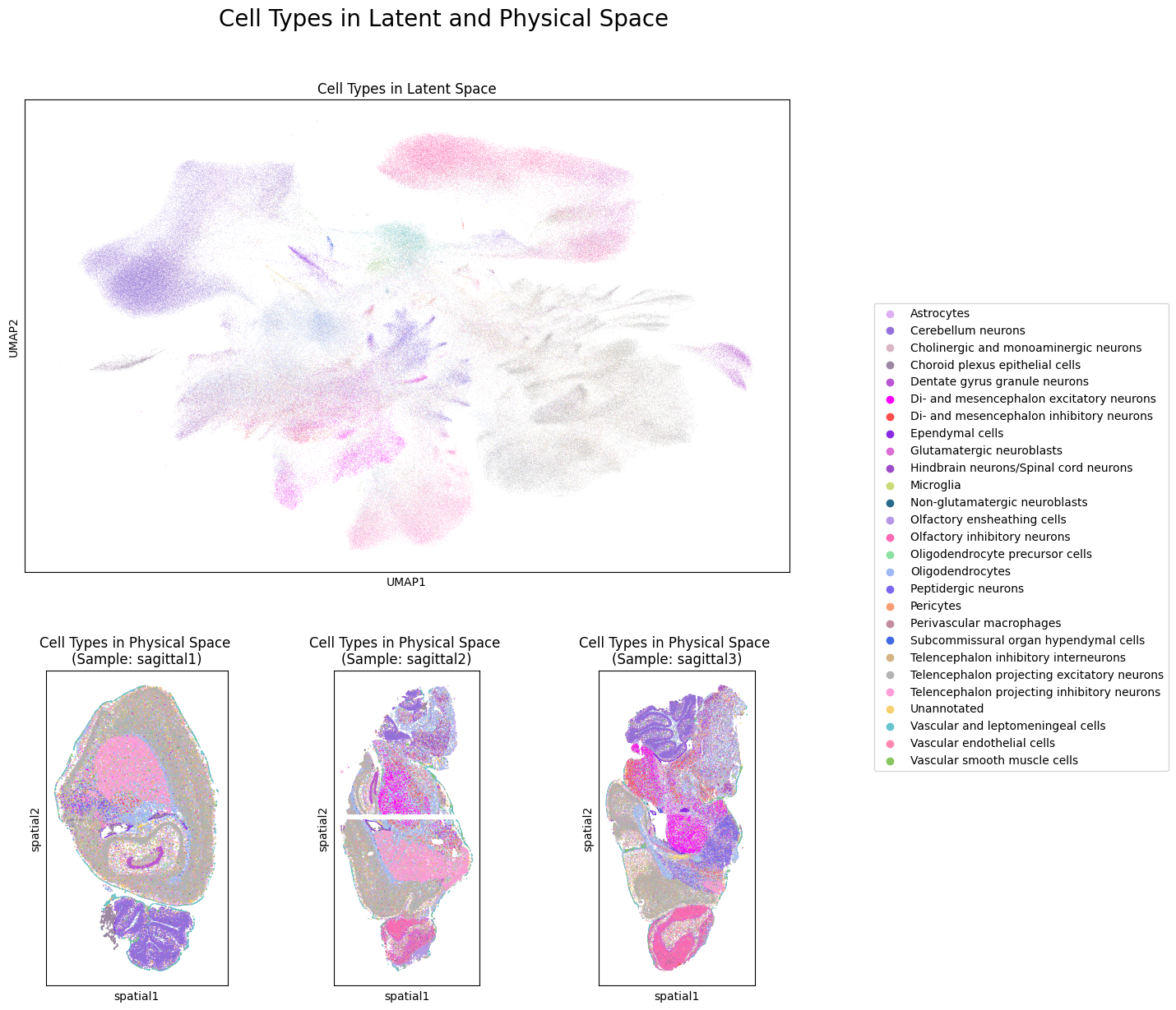
Next, let’s look at the preservation of cell type annotations in the latent GP space. Note that the goal of NicheCompass is not a separation of cell types but rather to identify spatially consistent cell niches.
# Create plot of cell type annotations in physical and latent space
groups = None
save_fig = True
file_path = f"{figure_folder_path}/" \
            "cell_types_latent_physical_space.svg"

fig = plt.figure(figsize=(12, 14))
title = fig.suptitle(t=f"Cell Types " \
                       "in Latent and Physical Space",
                     y=0.96,
                     x=0.55,
                     fontsize=20)
spec1 = gridspec.GridSpec(ncols=1,
                          nrows=2,
                          width_ratios=[1],
                          height_ratios=[3, 2])
spec2 = gridspec.GridSpec(ncols=len(samples),
                          nrows=2,
                          width_ratios=[1] * len(samples),
                          height_ratios=[3, 2])
axs = []
axs.append(fig.add_subplot(spec1[0]))
sc.pl.umap(adata=model.adata,
           color=[cell_type_key],
           groups=groups,palette=cell_type_colors,
           title=f"Cell Types in Latent Space",
           ax=axs[0],
           show=False)
for idx, sample in enumerate(samples):
    axs.append(fig.add_subplot(spec2[len(samples) + idx]))
    sc.pl.spatial(adata=model.adata[model.adata.obs[sample_key] == sample],
                  color=[cell_type_key],
                  groups=groups,
                  palette=cell_type_colors,
                  spot_size=spot_size,
                  title=f"Cell Types in Physical Space \n"
                        f"(Sample: {sample})",
                  legend_loc=None,
                  ax=axs[idx+1],
                  show=False)

# Create and position shared legend
handles, labels = axs[0].get_legend_handles_labels()
lgd = fig.legend(handles,
                 labels,
                 loc="center left",
                 bbox_to_anchor=(0.98, 0.5))
axs[0].get_legend().remove()

# Adjust, save and display plot
plt.subplots_adjust(wspace=0.2, hspace=0.25)
if save_fig:
    fig.savefig(file_path,
                bbox_extra_artists=(lgd, title),
                bbox_inches="tight")
plt.show()
4.2 Identify Niches
We compute Leiden clustering of the NicheCompass latent GP space to identify spatially consistent cell niches.
# Compute latent Leiden clustering
sc.tl.leiden(adata=model.adata,
             resolution=latent_leiden_resolution,
             key_added=latent_cluster_key,
             neighbors_key=latent_key)
latent_cluster_colors = create_new_color_dict(
    adata=model.adata,
    cat_key=latent_cluster_key)
# Create plot of latent cluster / niche annotations in physical and latent space
groups = None # set this to a specific cluster for easy visualization, e.g. ["0"]
save_fig = True
file_path = f"{figure_folder_path}/" \
            f"res_{latent_leiden_resolution}_" \
            "niches_latent_physical_space.svg"

fig = plt.figure(figsize=(12, 14))
title = fig.suptitle(t=f"NicheCompass Niches " \
                       "in Latent and Physical Space",
                     y=0.96,
                     x=0.55,
                     fontsize=20)
spec1 = gridspec.GridSpec(ncols=1,
                          nrows=2,
                          width_ratios=[1],
                          height_ratios=[3, 2])
spec2 = gridspec.GridSpec(ncols=len(samples),
                          nrows=2,
                          width_ratios=[1] * len(samples),
                          height_ratios=[3, 2])
axs = []
axs.append(fig.add_subplot(spec1[0]))
sc.pl.umap(adata=model.adata,
           color=[latent_cluster_key],
           groups=groups,
           palette=latent_cluster_colors,
           title=f"Niches in Latent Space",
           ax=axs[0],
           show=False)
for idx, sample in enumerate(samples):
    axs.append(fig.add_subplot(spec2[len(samples) + idx]))
    sc.pl.spatial(adata=model.adata[model.adata.obs[sample_key] == sample],
                  color=[latent_cluster_key],
                  groups=groups,
                  palette=latent_cluster_colors,
                  spot_size=spot_size,
                  title=f"Niches in Physical Space \n"
                        f"(Sample: {sample})",
                  legend_loc=None,
                  ax=axs[idx+1],
                  show=False)

# Create and position shared legend
handles, labels = axs[0].get_legend_handles_labels()
lgd = fig.legend(handles,
                 labels,
                 loc="center left",
                 bbox_to_anchor=(0.98, 0.5))
axs[0].get_legend().remove()

# Adjust, save and display plot
plt.subplots_adjust(wspace=0.2, hspace=0.25)
if save_fig:
    fig.savefig(file_path,
                bbox_extra_artists=(lgd, title),
                bbox_inches="tight")
plt.show()

4.3 Characterize Niches
Now we will characterize the identified cell niches.
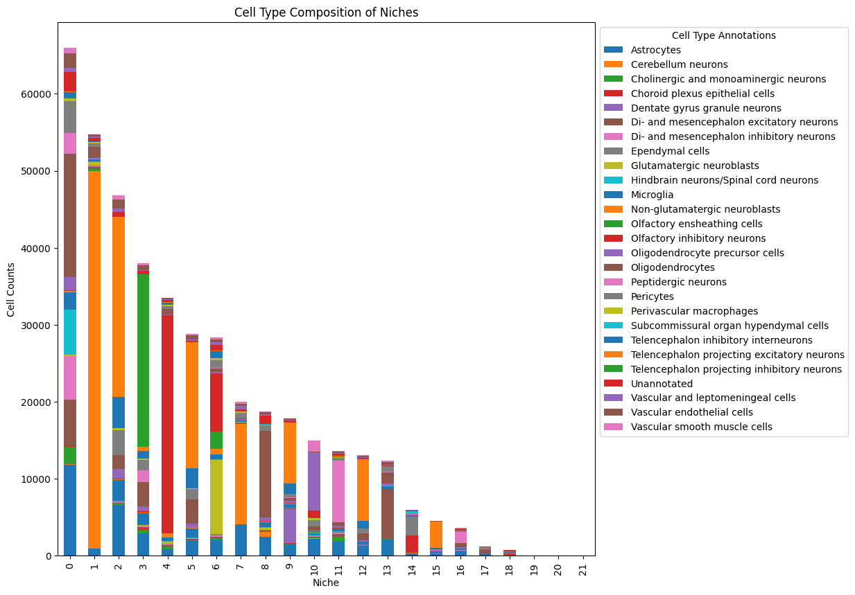
4.3.1 Niche Composition
We can analyze the niche composition in terms of batch and cell type labels.
save_fig = True
file_path = f"{figure_folder_path}/" \
            f"res_{latent_leiden_resolution}_" \
            f"niche_composition_batches.svg"

df_counts = (model.adata.obs.groupby([latent_cluster_key, cat_covariates_keys[0]])
             .size().unstack())
df_counts.plot(kind="bar", stacked=True, figsize=(10,10))
legend = plt.legend(bbox_to_anchor=(1, 1), loc="upper left", prop={'size': 10})
legend.set_title("Batch Annotations", prop={'size': 10})
plt.title("Batch Composition of Niches")
plt.xlabel("Niche")
plt.ylabel("Cell Counts")
if save_fig:
    plt.savefig(file_path,
                bbox_extra_artists=(legend,),
                bbox_inches="tight")

save_fig = True
file_path = f"{figure_folder_path}/" \
            f"res_{latent_leiden_resolution}_" \
            f"niche_composition_cell_types.svg"

df_counts = (model.adata.obs.groupby([latent_cluster_key, cell_type_key])
             .size().unstack())
df_counts.plot(kind="bar", stacked=True, figsize=(10,10))
legend = plt.legend(bbox_to_anchor=(1, 1), loc="upper left", prop={'size': 10})
legend.set_title("Cell Type Annotations", prop={'size': 10})
plt.title("Cell Type Composition of Niches")
plt.xlabel("Niche")
plt.ylabel("Cell Counts")
if save_fig:
    plt.savefig(file_path,
                bbox_extra_artists=(legend,),
                bbox_inches="tight")
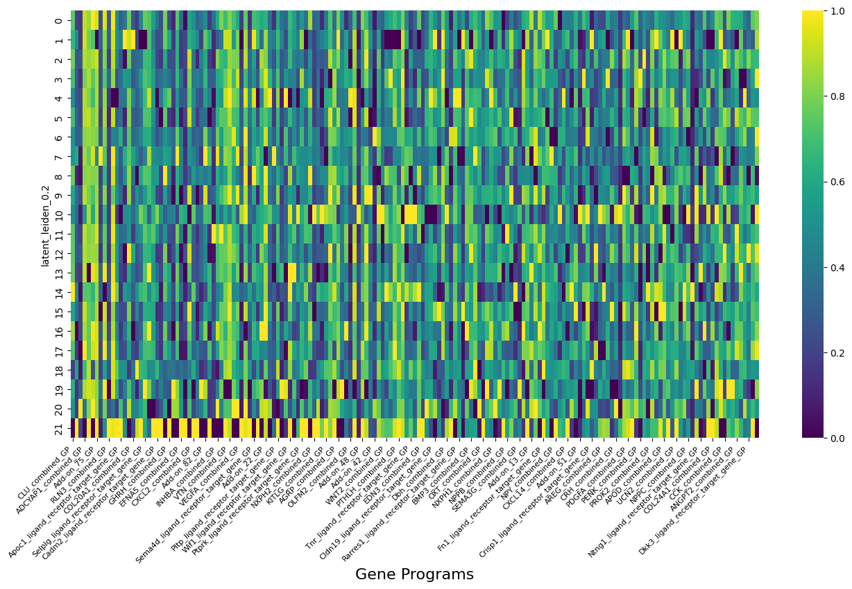
4.3.2 Differential GPs
Now we can test which GPs are differentially expressed in a niche. To this end, we will perform “one-vs-rest” differential GP testing, i.e all niches (selected_cats = None) are tested against all other niches (comparison_cats = "rest"). However, differential GP testing can also be performed in the following ways:
Set
selected_cats = ["0"]to perform differential GP testing for a specific niche only, in this case niche “0”.Set
comparison_cats = ["2"]to perform differential GP testing against niche “2” as opposed to against all other niches.
We choose an absolute log bayes factor threshold of 2.3 to determine strongly enriched GPs (see https://en.wikipedia.org/wiki/Bayes_factor).
# Check number of active GPs
active_gps = model.get_active_gps()
print(f"Number of total gene programs: {len(model.adata.uns[gp_names_key])}.")
print(f"Number of active gene programs: {len(active_gps)}.")
Number of total gene programs: 297.
Number of active gene programs: 230.
# Display example active GPs
gp_summary_df = model.get_gp_summary()
gp_summary_df[gp_summary_df["gp_active"] == True].head()
| gp_name | all_gp_idx | gp_active | active_gp_idx | n_source_genes | n_non_zero_source_genes | n_target_genes | n_non_zero_target_genes | gp_source_genes | gp_target_genes | gp_source_genes_weights | gp_target_genes_weights | gp_source_genes_importances | gp_target_genes_importances | |
|---|---|---|---|---|---|---|---|---|---|---|---|---|---|---|
| 0 | A2m_ligand_receptor_target_gene_GP | 0 | True | 0 | 1 | 1 | 32 | 32 | [A2M] | [A2M, PTHLH, RUNX1, SOCS3, JUNB, CCL3, CXCL1, ... | [-1.3424] | [-1.1694, 0.4261, 0.3762, 0.3034, -0.271, 0.23... | [0.1977] | [0.1722, 0.0627, 0.0554, 0.0447, 0.0399, 0.034... |
| 1 | Anpep_ligand_receptor_target_gene_GP | 1 | True | 1 | 1 | 1 | 31 | 31 | [ANPEP] | [NR2F2, VIM, SPP1, ZBTB20, LPL, GADD45A, TCF7L... | [0.1486] | [0.2963, 0.1976, -0.1884, 0.1837, -0.161, -0.1... | [0.0504] | [0.1004, 0.067, 0.0639, 0.0623, 0.0546, 0.0507... |
| 2 | Apoc1_ligand_receptor_target_gene_GP | 2 | True | 2 | 1 | 1 | 34 | 34 | [APOC1] | [IGF2, PTHLH, DKK1, VIM, NR2F2, BMP4, GATA3, V... | [0.3271] | [-1.1662, -0.355, 0.3373, 0.2653, -0.2597, -0.... | [0.0602] | [0.2148, 0.0654, 0.0621, 0.0489, 0.0478, 0.046... |
| 3 | C1qb_ligand_receptor_target_gene_GP | 3 | True | 3 | 1 | 1 | 31 | 31 | [C1QB] | [RUNX1, ADM, KRT15, TNF, SOCS3, BDNF, BRCA1, B... | [-1.5278] | [-0.5286, 0.3562, 0.2958, 0.259, -0.216, 0.165... | [0.3248] | [0.1124, 0.0757, 0.0629, 0.0551, 0.0459, 0.035... |
| 4 | Cadm1_ligand_receptor_target_gene_GP | 4 | True | 4 | 1 | 1 | 33 | 33 | [CADM1] | [CADM1, TAGLN, SNTB1, COL19A1, RGS4, CD9, FRZB... | [-0.8425] | [-0.8501, 0.4096, 0.3501, -0.2788, 0.2335, -0.... | [0.1662] | [0.1677, 0.0808, 0.0691, 0.055, 0.0461, 0.0437... |
# Set parameters for differential gp testing
selected_cats = None
comparison_cats = "rest"
title = f"NicheCompass Strongly Enriched Niche GPs"
log_bayes_factor_thresh = 2.3
save_fig = True
file_path = f"{figure_folder_path}/" \
            f"/log_bayes_factor_{log_bayes_factor_thresh}" \
             "_niches_enriched_gps_heatmap.svg"
# Run differential gp testing
enriched_gps = model.run_differential_gp_tests(
    cat_key=latent_cluster_key,
    selected_cats=selected_cats,
    comparison_cats=comparison_cats,
    log_bayes_factor_thresh=log_bayes_factor_thresh)
# Results are stored in a df in the adata object
model.adata.uns[differential_gp_test_results_key]
| category | gene_program | p_h0 | p_h1 | log_bayes_factor | |
|---|---|---|---|---|---|
| 0 | 21 | CLU_combined_GP | 0.000262 | 0.999738 | -8.247897 |
| 1 | 21 | DHH_combined_GP | 0.999258 | 0.000742 | 7.205151 |
| 2 | 20 | VIP_combined_GP | 0.999172 | 0.000828 | 7.096095 |
| 3 | 21 | ADCYAP1_combined_GP | 0.000859 | 0.999141 | -7.058946 |
| 4 | 13 | Add-on_44_GP | 0.000972 | 0.999028 | -6.935529 |
| ... | ... | ... | ... | ... | ... |
| 263 | 3 | PMCH_combined_GP | 0.089967 | 0.910033 | -2.314040 |
| 264 | 5 | Adenosine monophosphate_metabolite_enzyme_sens... | 0.090041 | 0.909959 | -2.313136 |
| 265 | 21 | Siglech_ligand_receptor_target_gene_GP | 0.090526 | 0.909474 | -2.307230 |
| 266 | 19 | Lefty1_ligand_receptor_target_gene_GP | 0.090595 | 0.909405 | -2.306397 |
| 267 | 21 | SEMA3F_combined_GP | 0.090847 | 0.909153 | -2.303342 |
268 rows × 5 columns
# Visualize GP activities of enriched GPs across niches
df = model.adata.obs[[latent_cluster_key] + enriched_gps].groupby(latent_cluster_key).mean()

scaler = MinMaxScaler()
normalized_columns = scaler.fit_transform(df)
normalized_df = pd.DataFrame(normalized_columns, columns=df.columns)
normalized_df.index = df.index

plt.figure(figsize=(16, 8))  # Set the figure size
ax = sns.heatmap(normalized_df,
            cmap='viridis',
            annot=False,
            linewidths=0)
plt.xticks(rotation=45,
           fontsize=8,
           ha="right"
          )
plt.xlabel("Gene Programs", fontsize=16)
plt.savefig(f"{figure_folder_path}/enriched_gps_heatmap.svg",
            bbox_inches="tight")
# Store gene program summary of enriched gene programs
save_file = True
file_path = f"{figure_folder_path}/" \
            f"/log_bayes_factor_{log_bayes_factor_thresh}_" \
            "niche_enriched_gps_summary.csv"

gp_summary_cols = ["gp_name",
                   "n_source_genes",
                   "n_non_zero_source_genes",
                   "n_target_genes",
                   "n_non_zero_target_genes",
                   "gp_source_genes",
                   "gp_target_genes",
                   "gp_source_genes_importances",
                   "gp_target_genes_importances"]

enriched_gp_summary_df = gp_summary_df[gp_summary_df["gp_name"].isin(enriched_gps)]
cat_dtype = pd.CategoricalDtype(categories=enriched_gps, ordered=True)
enriched_gp_summary_df.loc[:, "gp_name"] = enriched_gp_summary_df["gp_name"].astype(cat_dtype)
enriched_gp_summary_df = enriched_gp_summary_df.sort_values(by="gp_name")
enriched_gp_summary_df = enriched_gp_summary_df[gp_summary_cols]

if save_file:
    enriched_gp_summary_df.to_csv(f"{file_path}")
else:
    display(enriched_gp_summary_df)
Now we will have a look at the GP activities and the log normalized counts of the most important omics features of the differential GPs.
plot_label = f"log_bayes_factor_{log_bayes_factor_thresh}_cluster_{selected_cats[0] if selected_cats else 'None'}_vs_rest"
save_figs = True

generate_enriched_gp_info_plots(
    plot_label=plot_label,
    model=model,
    sample_key=sample_key,
    differential_gp_test_results_key=differential_gp_test_results_key,
    cat_key=latent_cluster_key,
    cat_palette=latent_cluster_colors,
    n_top_enriched_gp_start_idx=20,
    n_top_enriched_gp_end_idx=30,
    feature_spaces=samples, # ["latent"]
    n_top_genes_per_gp=3,
    save_figs=save_figs,
    figure_folder_path=f"{figure_folder_path}/",
    spot_size=spot_size)
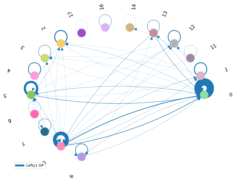
4.3.3 Cell-cell Communication
Now we will use the inferred activity of an enriched combined interaction GP to analyze the involved intercellular interactions.
gp_name = "Lefty1_ligand_receptor_target_gene_GP"
network_df = compute_communication_gp_network(
    gp_list=[gp_name],
    model=model,
    group_key=latent_cluster_key,
    n_neighbors=n_neighbors)

visualize_communication_gp_network(
    adata=model.adata,
    network_df=network_df,
    figsize=(9, 7),
    cat_colors=latent_cluster_colors,
    edge_type_colors=["#1f77b4"],
    cat_key=latent_cluster_key,
    save=True,
    save_path=f"{figure_folder_path}/gp_network_{gp_name}.svg",
    )